Build a line scan inspection system with Roboflow to detect defects on moving production lines. Select cameras and compute for your inspection requirements, then use Roboflow Workflows to process high-resolution images and validate results on your own materials.
A line scan inspection system requires three choices that constrain each other: the camera, the compute that runs inference, and the Workflow blocks that turn a high resolution image into defect detections. If you select the camera without considering compute, you can end up with a line that produces more image data than an edge device can inspect.
This guide covers the choices in the order they depend on each other. Your smallest defect sets the camera resolution. The camera and the Workflow settings together set how many tiles per second need inference. That number sets the compute.
How line scan cameras work
A line scan camera captures one row of pixels at a time similar to a flatbed scanner. As material moves past the sensor on a conveyor or rotary table, the rows stack into a continuous image. An area scan, by contrast, captures a full rectangular frame in one exposure similar to a point and shoot camera.
That makes line scan the standard choice for continuous surfaces and moving production lines: steel sheet, fabric rolls, printed labels, and coated films. The production process has no natural frame boundaries, and neither does the image. Since the line scan camera only captures a single row of pixels, a single exposure can capture more precise detail with less motion blur.
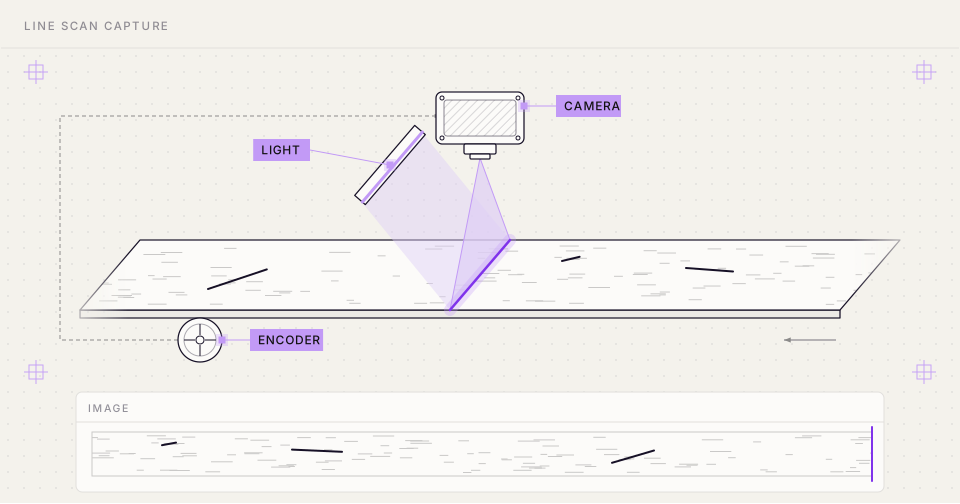
| Line scan | Area scan | |
|---|---|---|
| Capture | One line at a time, built up by motion | One 2D frame per exposure |
| Image shape | Fixed width, length set by how long you scan | Fixed width and height |
| Best for | Continuous webs, wide surfaces, rotating parts | Discrete parts, assemblies, static scenes |
| Motion | Required; line capture is synced to material travel | Frozen with short exposure or strobes |
| Lighting | A narrow, bright, uniform line | Even light across the whole field |
| Setup effort | Higher: encoder, sync, and alignment | Lower: point, trigger, shoot |
Step 1: Select the camera
Start from the defect. Four specs determine whether a camera can see your smallest defect at your line speed, and the interface limits how many of those lines reach the compute.
Specs that determine image quality
- Pixels per line: Divide the field of view by the number of pixels per line to get resolution across the material. A 4,096-pixel camera covering a 400 mm web resolves about 0.1 mm per pixel.
- Line rate: The camera’s line rate is the number of lines it captures per second. To keep pixels square, line rate must equal material speed divided by pixel size. At 2 m/s and 0.1 mm per pixel, that is 20,000 lines per second.
- Encoder triggering: An encoder on the conveyor triggers one line per fixed distance of travel. Without it, any speed change stretches or squashes the image, and your defects with it.
- Line lighting: Exposures are short (50 microseconds at 20 kHz), so the light must be intense and uniform along the scan line. If the lighting angle is wrong, a scratch may not appear.
Current 2k, 4k, and 8k cameras
Vendors sell resolution in steps: 2k (2,048 pixels per line), 4k (4,096), and 8k (8,192). Basler's current range is the racer 2 family, and LUCID's is the Triton line scan range, which gained an 8k model at VISION 2026. Compare the cameras in the table below on three points:
- The same sensor gives different line rates on different interfaces. The Basler 2k and 4k models and the LUCID Triton2 all use the Gpixel GL3504. At 4k it delivers 29 kHz over GigE, 65 kHz over 2.5GigE, and 84 kHz over 5GigE. The sensor did not change; the cable did because each interface carries a different amount of data per second.
- Color costs about half the line rate. Color versions of the Basler 4k models run at 14 kHz (GigE) and 42 kHz (5GigE, CXP-12). The color Triton2 runs at 33 kHz, and Basler's 8k color model runs at 80 kHz.
- At 8k, the two vendors use different interfaces. Basler's 8k needs CoaXPress and a frame grabber. LUCID's reaches 8k over standard 10GigE at a lower line rate. Basler also offers 16k at up to 120 kHz.
Published maximum line rates for the mono versions, as of November 2026:
Bandwidth limits
Every line the camera captures has to travel down the cable, so the data rate is pixels per line × bits per pixel × line rate. The interface puts a ceiling on that product: raise one factor, and another has to come down.
Take the Basler 4k GigE camera. Its sensor can run at 84 kHz, but 4,096 pixels × 8 bits × 29,000 lines per second is 950 Mbit/s, which fills a 1 Gbit/s link. So Basler rates the camera at 29 kHz. It rates the 2k version on the same link at 58 kHz: half the pixels, twice the lines, and the same 950 Mbit/s. Each interface sets a different ceiling:
| Interface | Approximate ceiling | What it carries |
|---|---|---|
| GigE | 1 Gbit/s | 4k mono at 29 kHz, or 2k at 58 kHz |
| 2.5GigE | 2.5 Gbit/s | 4k mono at 65 kHz |
| 5GigE | 5 Gbit/s | 4k mono at 84 kHz (now sensor-limited, about 2.8 Gbit/s) |
| 10GigE | 10 Gbit/s | 8k mono at 55 kHz (about 3.6 Gbit/s) |
| CXP-12 | 12.5 Gbit/s per link, up to 25 Gbit/s on racer 2 L | 8k mono at 240 kHz (about 15.7 Gbit/s at 8 bits) |
Pixel format and line rate
Pixel format sets the bits per pixel, so it moves the line rate ceiling directly. For a 4k camera on GigE, with roughly 950 Mbit/s to spend, every extra bit costs lines per second:
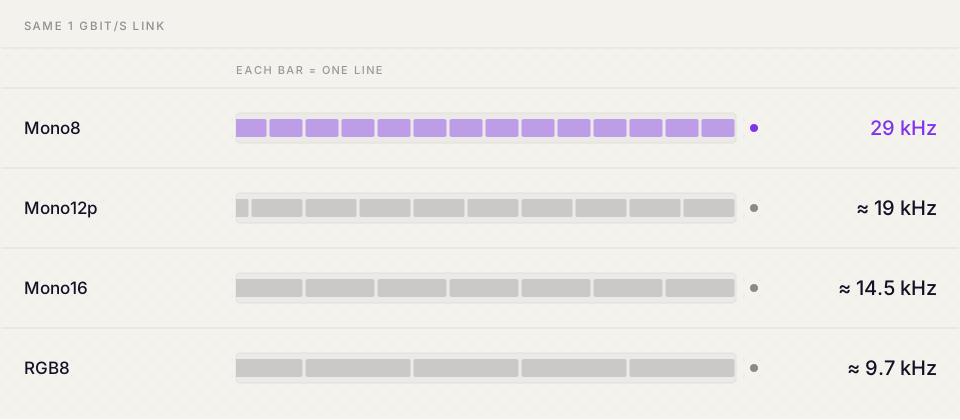
In the table below, the Mono8 row is Basler's published figure. The other rows divide the same budget by the bits per pixel, and they match Basler's published 14 kHz for the 4k color GigE model.
| Pixel format | Bits per pixel on the wire | Maximum line rate | Maximum web speed at 0.1 mm per pixel |
|---|---|---|---|
| Mono8 | 8 | 29 kHz | 2.9 m/s |
| Mono12 packed | 12 | about 19 kHz | 1.9 m/s |
| Mono10 or Mono12 unpacked | 16 | about 14.5 kHz | 1.45 m/s |
| YCbCr422 (color) | 16 | about 14.5 kHz | 1.45 m/s |
| RGB8 (color) | 24 | about 9.7 kHz | 0.97 m/s |
Rules for specifying a camera
- Use Mono8 unless you have a reason not to. Detection models take 8-bit images. Sending 12-bit data halves your line rate on a saturated link, and the extra bits are discarded before inference.
- Pick resolution from your smallest defect. Work out the pixel size you need for your smallest defect, then the pixels per line to cover the web. Going from 4k to 8k halves the line rate on the same link and roughly doubles the tiles to run: 9 across at 4k, 17 at 8k.
- Check which limit you are hitting. On GigE, the cable is the limit. On 5GigE and faster links, the sensor is often the limit, and a faster interface gains nothing.
- Check the conditions behind published rates. Published rates assume single-line readout, minimum exposure, jumbo packets, and a dedicated link. LUCID's 8k drops from 55 to 33 kHz in two-line mode. A narrower region of interest raises the ceiling again.
Step 2: Choose the Workflow blocks
The camera limits how much image data arrives. Your Workflow sets how it gets inspected. Detection models expect a small, roughly square input, so the blocks you choose have to fit a strip thousands of pixels long into a model that sees a few hundred pixels at a time.
Resizing versus tiling
Detection models take a fixed, roughly square input a few hundred pixels per side. A line scan strip can be thousands of pixels wide and far longer. If you resize a 4,096x20,000 strip to 640 pixels on its long side, a 30-pixel scratch becomes about one pixel, which is too small for the model to detect.
Instead, keep every pixel and cut the image into tiles. Each of the following steps fixes a problem that the previous step creates:
- Tile: Slice the strip into model-sized tiles and run inference on each. Every defect keeps its full resolution. But a cut line can split a defect between two tiles, so the model sees two fragments instead of one defect.
- Overlap: Make neighboring tiles share a margin. A defect on a boundary now appears whole in at least one tile, provided the defect is smaller than the margin. But the model detects anything inside the margin twice.
- Stitch: Shift each tile's boxes back into strip coordinates, then run non-maximum suppression (NMS). Where two boxes overlap beyond a threshold, NMS keeps the more confident one.
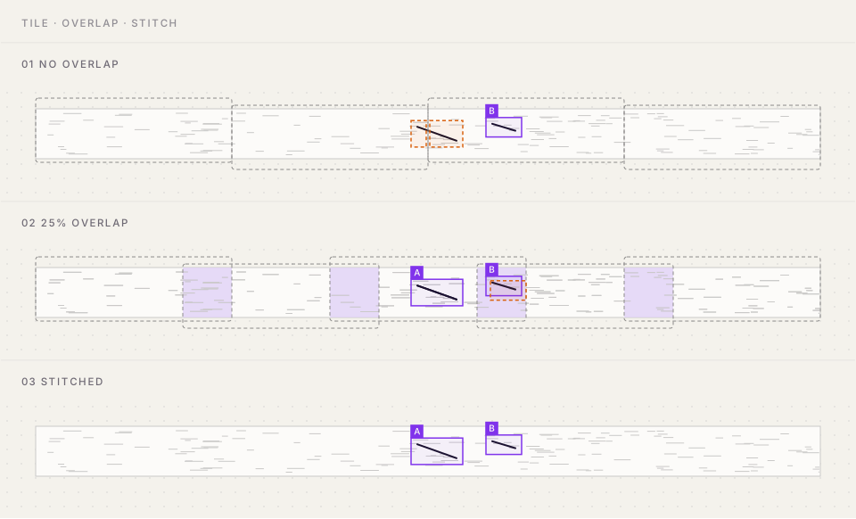
Overlap protects only defects that are smaller than the overlap. A long scratch that crosses several tiles still comes back as several boxes, one per tile. If your defects are long, use a larger overlap, larger tiles, or a merge-based filter instead of NMS, as described in Choose the settings.
The blocks you need
The pipeline is three blocks in Roboflow Workflows, plus two visualization blocks to draw the result.
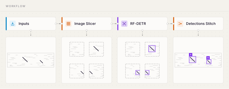
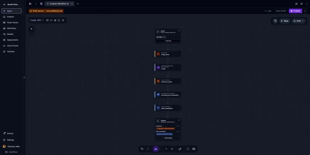
Image Slicer
Image Slicer cuts the strip into overlapping tiles. Set the slice width and height to 640 and both overlap ratios to 0.25.
With these settings, each tile shares 160 pixels with its neighbor, and the slicer advances 480 pixels per tile. Any defect narrower than 160 pixels appears whole in at least one tile.
Object Detection Model
Connect the model block to the slicer’s output. The model runs once per tile and returns a separate set of predictions for each. The model treats each tile as an ordinary image.
Train the model on tiles cut from your strips: it only ever sees single tiles, so it needs to work well at tile scale and production resolution. The screenshots in this section use a Pill Detection project as the example: 496 images of individual tablets and capsules, with a model that reached 99.5% mAP on the validation set.
Detections Stitch
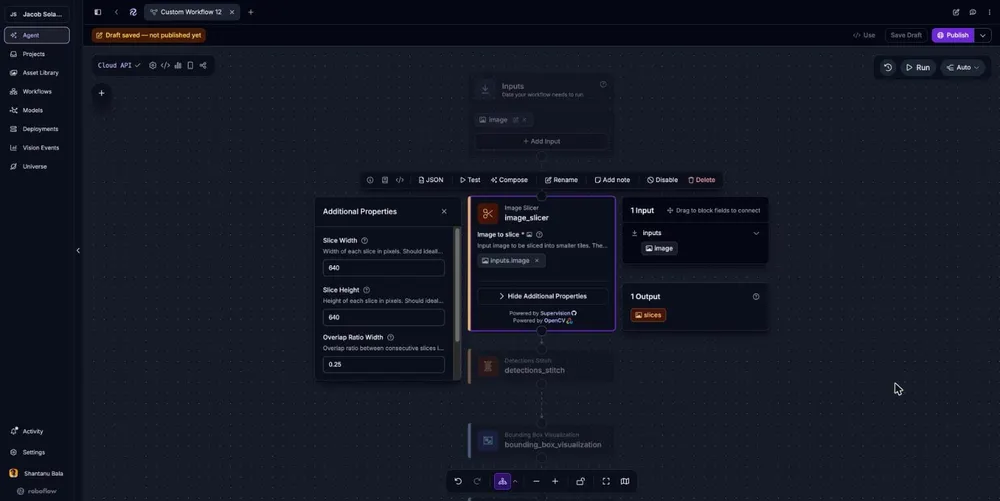
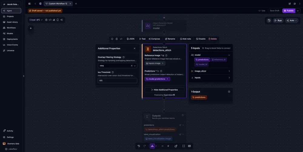
Detections Stitch takes the per-tile predictions plus the original strip as a reference. It shifts every box from tile coordinates to strip coordinates, then filters duplicates. Set the overlap filtering strategy to NMS and the IoU threshold to 0.5.
Visualization
Finally, Bounding Box Visualization and Label Visualization draw the merged detections on the full strip. The Workflow returns both the annotated image and the prediction list.
Choose the settings
| Setting | Starting value | How to choose it for your line |
|---|---|---|
| Tile size | 640x640 | Pick the size at which defects appear at the same pixel scale as in your training images |
| Overlap | 0.25 (160 px) | At least the pixel size of the largest defect you need returned as a single box |
| Filtering strategy | NMS | NMS for compact defects; non-max merging for long defects that span tiles |
| IoU threshold | 0.5 | Lower it if duplicates survive; raise it if nearby distinct defects get merged |
Validate the combination
Run strips from your own camera through the Workflow. One call slices the strip, detects on every tile, and returns a single set of boxes in strip coordinates.
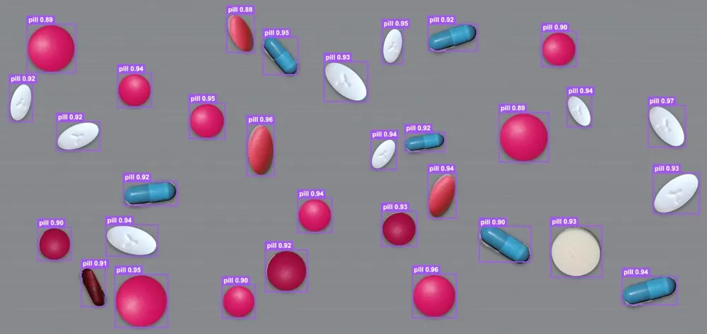
Check the output for:
- Coverage: Detections appear along the whole strip.
- Boundaries: Defects that sit across a tile edge come back as one complete box.
- Duplicates: Defects inside an overlap zone have one box.
Step 3: Choose the compute
Every tile is one model call, so tiles per second is the load the device has to carry. With 640-pixel tiles at 0.25 overlap and square frames:
| Camera and link | Line rate | Square frames per second | Tiles per frame | Tiles per second |
|---|---|---|---|---|
| 2k Mono8 on GigE | 58 kHz | 28.3 | 16 | about 450 |
| 4k Mono8 on GigE | 29 kHz | 7.1 | 81 | about 570 |
| 4k Mono8 on 5GigE | 84 kHz | 20.5 | 81 | about 1,660 |
| 8k Mono8 on 10GigE | 55 kHz | 6.7 | 289 | about 1,940 |
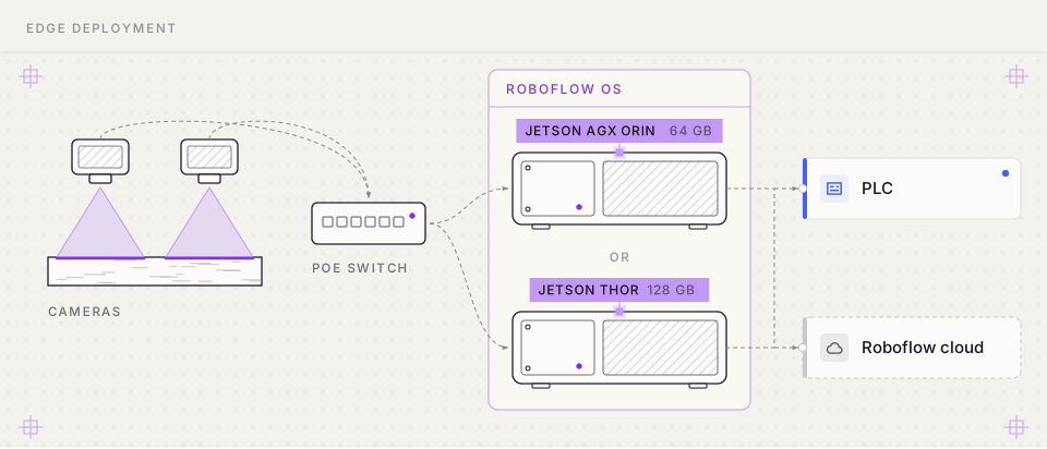
Roboflow OS runs on Jetson AGX Orin 64 GB and Jetson Thor T5000 128 GB. Thor connects over QSFP28 (4 × 25GbE) but has no Power over Ethernet (PoE) ports, so the cameras draw power from a PoE switch.
Check the device against the load
Every tile is a full model run, so these loads are demanding for a single edge device. Before you commit to hardware, run your Workflow on the device with tiles from your own line and measure how many tiles per second it sustains, including slicing and stitching. Compare that figure to the load for your camera.
If the device falls short, you have four levers:
- Bigger tiles or less overlap: Fewer tiles per frame means fewer model runs. Check that defects still appear at the scale the model was trained on, and that the overlap still covers your largest defect.
- A narrower region of interest or a slower line: Inspect only the part of the web that matters, or lower the line rate by running the material more slowly.
- A smaller or faster model: Use a smaller model size, or export it to TensorRT at reduced precision, then confirm accuracy on your boundary test set.
- More devices: Split the cameras, or divide the web into lanes, across several devices.
Plan for a continuous line
A production line differs from a single test strip in four ways. Plan for each before you deploy.
- Continuous strips: A camera does not hand you one finished image. Your acquisition software cuts the stream into frames of a fixed number of lines. Overlap consecutive frames the same way you overlap tiles. Otherwise, a frame boundary splits defects, and comes back as two partial detections.
- Training scale: A model trained on tiles where a scratch is 40 pixels long struggles when production tiles show it at 120 pixels. Train on tiles cut from real strips at production resolution, and slice at that same size.
- Tile count: At 640-pixel tiles with 25% overlap, a 4,096-pixel-wide strip needs 9 tiles across. A 4,096x4,096 frame is 81 inferences. Check that against your line speed, and reduce overlap or increase tile size if you need headroom.
- Boundary testing: A model can score well on overall mAP and still miss defects at tile edges. Build a test set of defects that fall on tile and frame boundaries, and compare the output against a reference inspection.
Build your line scan inspection system
The right combination starts from the defect. Choose the pixel size that resolves it, the camera and link that deliver that resolution at your line speed, the tile and overlap settings that keep defects whole, and an edge device that keeps up with the resulting tiles per second. The Workflow itself stays the same three blocks.
To adapt it, swap in strips from your own camera and a model trained on your materials, then tune tile size and overlap against defects you already know about.
Build your inspection pipeline in Roboflow Workflows, and test it on your own images.
Further reading