AI/ML News & Innovations Hub

AI/ML news, top picks, and generated innovation digests.

★ Visit ai-karthik.com
422Sources
23769News Items
8Top Picks
148Blogs
failedLast Run

Latest AI/ML News

23769 matching items

How to calculate proportion of the population
Cross Validated 2021-03-25 03:22 UTC Score 12.0 AI-113-20210325-social-media-4728379e Full article

How to calculate proportion of the population

I am trying to calculate population attributable fraction. The formula that i am using is $$ \frac{P_e(RR-1)}{P_e(RR-1) + 1} $$ I am using this website as guide: https://sphweb.bumc.bu.edu/otlt/mph-modules/ep/ep713_association/EP713_Association7.html I am unable to understand how did they calculate $P_e$ . It says that its proportion of exposed subjects in entire population. The entire population here is 100,000 and total exposed subjects are 10,000 (500 with disease and 9500 without disease). If i do $10000/100000$ then the answer is $0.1$ . How did the website shows its $0.2$ ?

Lilian Weng Blog 2021-03-21 00:00 UTC Score 39.0 USR-0112-20210321-ai-specialis-3e60cc8a Full article

Reducing Toxicity in Language Models

Large pretrained language models are trained over a sizable collection of online data. They unavoidably acquire certain toxic behavior and biases from the Internet. Pretrained language models are very powerful and have shown great success in many NLP tasks. However, to safely deploy them for practical real-world applications demands a strong safety control over the model generation process.

AI Stack Exchange 2021-03-11 13:04 UTC Score 14.0 AI-110-20210311-social-media-275c4d77

How to define a "don't care" class in time series classification in Pytorch?

This is a theoretical question. Setup I have a time series classification task in which I should output a classification of 3 classes for every time stamp t . All data is labeled per frame. The problem: In the data set are more than 3 classes [which are also imbalanced]. My net should see all samples sequentially, because it uses that for historical information. Thus, I can't just eliminate all irrelevant class samples at preprocessing time. In case of a prediction on a frame which is labeled differently than those 3 classes, I don't care about the result. My thoughts: The net will predict for 3 classes The net will only learn (pass backward gradient) for valid classes, and just not calculate loss for other classes. Questions Is this the way to go for "don't care" classes in classification? How to calculate loss only for relevant classes in Pytorch? Should I apply some normalization per batch, or change batch norm layers if dropping variable samples per batch? I am using nn.CrossEntropyLoss() as my criterion, which has only mean or sum as reductions. I need to mask the batch so that the reduction will only apply for samples whose label is valid. I could use reduction='none' and do that manually, or I could do that before the loss and keep using reduction='mean' . Is there some method to do this using built in Pytorth tools? Maybe this can be done in the data-fetching phase somehow? I am looking some standard, vanilla, thumb rule implementation to tackle this. The least fancy…

Cross Validated 2021-03-10 17:24 UTC Score 15.0 AI-113-20210310-social-media-9ca2fbb8

Forecast accuracy of simulation vs empirical measurement

I want to compare how well a simulated curve approximates the "real" curve measured on empirical data. More in detail: I have empirical data, let's say for simplicity the worldwide population per year for the last 200 years. I measure a curve that is mostly increasing with 1 data point for each year. Now I also have a model with some parameters that I use to simulate the same curve. For the simulation I only use the starting point (population at the first year) as well as some universal parameters that I can estimate from any time span in the empirical data and that don't change in time. So I end up with two curves, the real one and the simulated one. Now I want to quantify how accurate my simulation is compared to the empirical data. How would I approach this apart from plotting both curves on top of each other? Are measures like Mean absolute percentage error or scaled errors the right way? As I am very new to this topic I apologize if this is perhaps a very trivial or stupid question

Proper way to perform cross-validatation for selecting best parameters to build a calibrated model and assessing the error of the model?
Cross Validated 2021-03-10 05:33 UTC Score 15.0 AI-113-20210310-social-media-90736b7e Full article

Proper way to perform cross-validatation for selecting best parameters to build a calibrated model and assessing the error of the model?

I want to find the best possible: Post process to apply on my data (for example, whether or not perform PCA or scaling, to remove some features...). Some of this options have parameters to tune (like number of components). Model. Hyperparameters of the model. I want also to assess or validate how good is the model. To find those, I thought of performing a double nested Cross Validation. The problem is that I want a calibrated model, and calibration needs new unseen data to be trained on. So I am not fully sure how to implement it.

Writing MA and AR representations
Cross Validated 2021-03-09 20:22 UTC Score 10.0 AI-113-20210309-social-media-c2a6e003 Full article

Writing MA and AR representations

I have to determine if $$(1 - 1.1B + 0.8B^2)Y_t = (1 - 1.7B + 0.72B^2)a_t$$ is stationary, invertible or both. I have shown that $\Phi(B) = 1 - 1.1B + 0.8B^2 = 0$ when $B_{1,2} = 0.6875 \pm 0.8817i$ , whose moduli are both larger than 1, hence is stationary. Similarly, I have shown that $\Theta(B) = 1 - 1.7B + 0.72B^2 = 0$ , when $B_1 = 1.25 > 1$ and $B_2 = 1.11 > 1$ , hence is invertible. I also need to express the model as a MA and AR representation if it exists; which they do as I have already shown. However, to write as an MA process, I would need to write as: $$Y_t = \frac{1 - 1.7B + 0.72B^2}{1 - 1.1B + 0.8B^2}a_t$$ and for an AR process as: $$\frac{1 - 1.1B + 0.8B^2}{1 - 1.7B + 0.72B^2}Y_t = a_t$$ However, I am confused on how to do this given the division of the quadratic expressions. Should I use long division or is there some expansion formula I should be using?

Should dummy variables be allowed to correlate (R code & data provided)
Cross Validated 2021-03-07 18:32 UTC Score 12.0 AI-113-20210307-social-media-d484c114 Full article

Should dummy variables be allowed to correlate (R code & data provided)

tl;dr: What is the difference between a regression model that allows its dummy variables to be correlated and one that doesn't do so? For example, how does that affect Standard Error of the regression coefficients (coefs)? In my reproducible SEM ( structural equation model ) modelA below, imagine I remove the Group_HI ~~ 0*Group_MT (denoting correlation bet. two dummies is 0 ) altogether leading to modelB . What is the difference between a model that uses Group_HI ~~ 0*Group_MT ( modelA ) and one that doesn't include anything to describe the relation between Group_HI and Group_MT ( modelB )? Specifically, it seems modelB produces Standard Errors for coefs that are closer to those given by a MANOVA: summary(lm(cbind(MP,SE)~Group,data=d)) Response MP : Estimate Std. Error t value Pr(>|t|) (Intercept) 4.6667 0.6150 7.588 8.19e-10 *** GroupHI 3.1833 0.8136 3.913 0.000281 *** ## This SE GroupMT 6.7451 0.8438 7.994 1.95e-10 *** ## This SE Response SE : Estimate Std. Error t value Pr(>|t|) (Intercept) 4.2000 0.3378 12.432 But modelA produces Standard Errors for coefs that are closer to those given by: stacked_DVs |t|) DVMP 4.666667 0.4961705 9.405370 2.364383e-15 DVSE 4.200000 0.4961705 8.464833 2.559422e-13 GroupHI 3.183333 0.6563718 4.849893 4.648941e-06 ## This SE GroupMT 6.745098 0.6807403 9.908475 1.912183e-16 ## This SE Reproducible data and R code: library(tidyverse); library(fastDummies) ; library(lavaan) d |z|) MP ~ Group_HI 3.183 0.659 4.830 0.000 ## This SE SE ~ Group_HI…

Can the law of iterated expectation be used on the inner expectation of the DQN cost function described in the DQN paper
AI Stack Exchange 2021-03-04 12:04 UTC Score 17.0 AI-110-20210304-social-media-d2ba293b Full article

Can the law of iterated expectation be used on the inner expectation of the DQN cost function described in the DQN paper

Is the expression for the DQN cost function, Equation (2) of the DQN paper $$\begin{align}L_1 &= E_{\mu,\pi}\left[\left(y_i - q(s,a;\theta)\right)^2\right]\\ &=E_{\mu,\pi}\left[\left(E_{\mathcal{E}}[r + \gamma \max\limits_{a'}q(s',a';\theta^-)] - q(s,a;\theta)\right)^2\right] \end{align}$$ equivalent to this? (Substituting the expression for $y_i$ defined in the paragraph directly after, $\mathcal{E}$ represents the transition distribution governed by the environment, $\pi$ represents the behaviour policy and $\mu$ represents the stationary distribution of states) $$L_2 = E_{\mu,\pi,\mathcal{E}}\left[\left(r + \gamma \max\limits_{a'}q(s',a';\theta^-) - q(s,a;\theta)\right)^2\right]$$ Can the law of iterated expectation be used to derive the second expression from the first, if not, is there another way to go about showing their equivalence IF they are equivalent. It seems as though $L_2$ is used for sampling but I'm not sure how it's possible to get here from the original cost function $L_1$ . If it is possible to use $L_2$ to sample I assume that means the two expressions must be equivalent. The second expression is used for sampling in the DQN paper here. I do realise that the gradient for each function is the same and thus so is the $n^{th}$ derivative for some $n\geq1$ and since the curvature and optimas align I guess that also means they are the same function (minus some constant difference)? $$\nabla_{\theta} L = E_{\mu,\pi,\mathcal{E}}\left[\left(r + \gamma \max\limit…

How to Speed Up Pandas with Modin
Anyscale Blog 2021-03-03 00:00 UTC Score 35.0 USR-0085-20210303-ai-specialis-34d3e5fb Full article

How to Speed Up Pandas with Modin

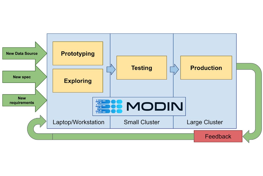
The pandas library provides easy-to-use data structures like pandas DataFrames as well as tools for data analysis. One issue with pandas is that it can be slow with large amounts of data. It wasn’t designed for analyzing 100 GB or 1 TB datasets. Fortunately, there is the Modin library which mitigates these issues.

Oxford Machine Learning Research Group 2021-03-01 17:41 UTC Score 25.0 USR-0027-20210301-research-aca-79a93137 Full article

aistats_iclr_2021

AISTATS and ICLR acceptances 2021 Alexander Camuto, Matthew Willetts, Brooks Paige, Chris Holmes and Stephen Roberts (2021). Learning Bijective Feature Maps for Linear ICA. Proceedings of AISTATS 2021 (to appear). Alexander Camuto, Matthew Willetts, Stephen Roberts, Chris Holmes, Tom Rainforth (2021).

Diff-in-Diff with a binary outcome? (i.e., comparing proportions of two groups over two time points in a paired setting)
Cross Validated 2021-03-01 17:33 UTC Score 15.0 AI-113-20210301-social-media-e21897ed Full article

Diff-in-Diff with a binary outcome? (i.e., comparing proportions of two groups over two time points in a paired setting)

Let's say I have students randomly split into two groups (treatment and control). Each student is given a test and they either pass or fail. They then either take a course (the students in "treatment") or they don't (students in "control") - then they take the exam again. I want to know if the course helped the students who took the exam in the second time. If we had only the second time, and wanted to compare treatment to control, we could use Chi-square test (or Fisher's exact test). If we had only one group (e.g., treatment), and we wanted to compare the success in the example before-after the course, we could have used McNemar's test. But what test would I use to compare the effect of the course on the improvement in the exam's pass rates? If the outcome wasn't pass/fail, but a normal outcome, we could have taken the difference between the before and after for each student, and then compare the two groups using a two sample $t$ -test (i.e., Diff-in-Diff). But how should I proceed with a binary outcome?

Differencing in a simple OLS regression
Cross Validated 2021-02-25 21:19 UTC Score 12.0 AI-113-20210225-social-media-6348763c Full article

Differencing in a simple OLS regression

I am attempting to do a simple OLS regression on time series data from 1990 to 2019, and there are trends in my variables: GDP per capita (dependent variable), oil prices, etc., which I can difference. I cannot difference variables such as inflation, as they are already stationary, as demonstrated on Eviews. Is it acceptable in a model to have differenced variables and variables which are already stationary and if so, why? For context I am using log( gdp per capita) as my dependent variable, with oil price as my primary independent in combination with net exports and inflation to calculate the impact of oil price on a net exporting country. I am unable to conduct (S)VAR analysis as I have not been taught this yet. Any further help would be greatly appreciated.

Checking significance in differences between groups (gaps in income between genders and education levels)
Cross Validated 2021-02-24 11:01 UTC Score 9.0 AI-113-20210224-social-media-22671c95 Full article

Checking significance in differences between groups (gaps in income between genders and education levels)

I wonder if you could give me a hint on how to find out whether there is a significant difference in the income gap between genders and their education level. The picture below shows education levels (edu_level_old), means for women and men income (in Russian currency), and a gap in income measured by %. I had no problem with finding out whether, for example, women with higher education earn less than men with higher education (done this by ttest). BUT what I would like to discover is whether this gap in earnings between different education levels (for example, a gap between those with higher education and secondary education) is statistically different . Is there a way I could do that? I have a feeling that it is rather simple and obvious for some but have no idea how to accomplish that. Your help is much appreciated!

Late Onset Augmentation
AI Stack Exchange 2021-02-16 20:43 UTC Score 16.0 AI-110-20210216-social-media-45ad770b Full article

Late Onset Augmentation

If I train a U-Net model for image segmentation (e.g. medical images) and start training until it converges and then add augmentation - can i expect similar results as if i train with augmentation from the beginning ?

Data Processing Support in Ray
Anyscale Blog 2021-02-16 00:00 UTC Score 30.0 USR-0085-20210216-ai-specialis-40161c22 Full article

Data Processing Support in Ray

This blog post highlights two features in the latest Ray 1.2 release: native support for spilling to external storage, and support for libraries from the Python data processing ecosystem, including integrations for PySpark and Dask.

Distill Archive 2021-02-11 20:00 UTC Score 10.0 AI-038-20210211-ai-specialis-e4474d4a Full article

Self-Organising Textures

Neural Cellular Automata learn to generate textures, exhibiting surprising properties.

Data Science Stack Exchange 2021-02-11 19:29 UTC Score 29.0 AI-111-20210211-social-media-43792a8a Full article

Train MLP Neural Network on time series data?

Newbie question here but I was curious to ask if an MLP Neural type network can be trained on time series data? The dataset that I have is an electricity type data set from a building power meter and I can find I can train a decent NN model with including a lot of weather data and also a lot of one hot encoding dummy variables for time-of-week. (day, hour, month number, etc.) I am experimenting in Python with the Tensorflow Keras library and I know the default during the training process randomly shuffles the data. Is this a No-No for a time series type problem where the random shuffle will take out the seasonality from the data? (stationary/non-stationary) The results shuffling the data really aren't that bad at a glance but not-randomly shuffling the data the results for MLP NN are poor, like the model doesn't train well. I know some other times series forecast methods can include ARIMA, LSTM, etc. but I was curious to inquire if MLP can be used for these purposes too? What I ultimately need is a short term forecast method that can incorporate hourly weather forecast (from a web API) to forecast future hourly building electricity. Any tips greatly appreciated. Thanks

Is there any statistically meaningful definition for object confidence in object detection?
Cross Validated 2021-02-09 14:50 UTC Score 12.0 AI-113-20210209-social-media-46aef6a3 Full article

Is there any statistically meaningful definition for object confidence in object detection?

Most modern object detection algorithms rely on neural networks and output a bounding box and confidence for each object (or more accurately, a confidence for each possible object class considered, the highest of which is taken to be the true object confidence and to define the predicted class for that object). Beyond giving a relative likelihood of "objectness" (a predicted bounding box with 0.9 confidence is more likely to actually contain an object than a predicted bounding box with 0.1 confidence), is there any statistical significance to these predictions? For instance, should we be able to say that a predicted confidence of 0.1 indicates that roughly 10% of predictions at this confidence are actually objects? Is there another statistically meaningful definition? I understand that at best this would be a loose statistical meaning because neural networks would be trained with loss functions that codify this statistical distribution into a loss, and the network would then only approximate this statistical distribution. Thus the distribution would also depend on the loss function used to train the classification portion of the neural network. These issues notwithstanding, is there or was there at some point inherent meaning to the confidence measure, or is it purely a relative quantity?

Why does Chinese Restaurant Table Distribution look like a Gaussian Distribution?
Cross Validated 2021-02-09 03:18 UTC Score 9.0 AI-113-20210209-social-media-616459ea Full article

Why does Chinese Restaurant Table Distribution look like a Gaussian Distribution?

The Chinese Restaurant Table Distribution describes the probability distribution for the number of non-empty tables in the Chinese Restaurant Process after $T$ customers have been seated. Specifically, if $K_T$ is the (random) number of non-empty tables after seating $T$ customers in a $CRP(\alpha)$ , its PMF is defined as $$P(K_T = k) = \frac{\Gamma(\alpha)}{\Gamma(\alpha + T)} |S(T, k)| \alpha^k$$ where $k \in \{1, ..., T\}$ and $|S(\cdot, \cdot)|$ are unsigned Stirling numbers of the first kind. I discovered that when I fix $\alpha$ and plot the distribution for increasing values of $T$ , the distribution looks more and more like a Gaussian. For alpha=10.01, I plot the distribution from T=1 (red) to T=50 (blue): My question is: why does the Chinese Restaurant Table distribution look like a Gaussian distribution for medium-to-large $T$ ?

Distill Archive 2021-02-04 20:00 UTC Score 10.0 AI-038-20210204-ai-specialis-a9b7e7bb Full article

Visualizing Weights

We present techniques for visualizing, contextualizing, and understanding neural network weights.

fAIr LAC 2021-02-03 14:10 UTC Score 27.0 USR-0219-20210203-ai-specialis-69725fc4 Full article

fAIr LAC: Adopción ética y responsable de la inteligencia artificial en América Latina y el Caribe

fAIr LAC: Adopción ética y responsable de la inteligencia artificial en América Latina y el Caribe @administrador Mié, 03/02/2021 - 14:10 Adopción ética y responsable de la inteligencia artificial en América Latina y el Caribe Imagen principal Categoría Publicaciones Tipo de recurso Documentos Archivos de recurso Prueba de nota técnica Descargar Enlace externo https://publications.iadb.org/es/fair-lac-adopcion-etica-y-responsable-de-la-in… Destacado Desactivado Order destacado -1

How to Speed up Scikit-Learn Model Training
Anyscale Blog 2021-02-03 00:00 UTC Score 36.0 USR-0085-20210203-ai-specialis-11e59c6e Full article

How to Speed up Scikit-Learn Model Training

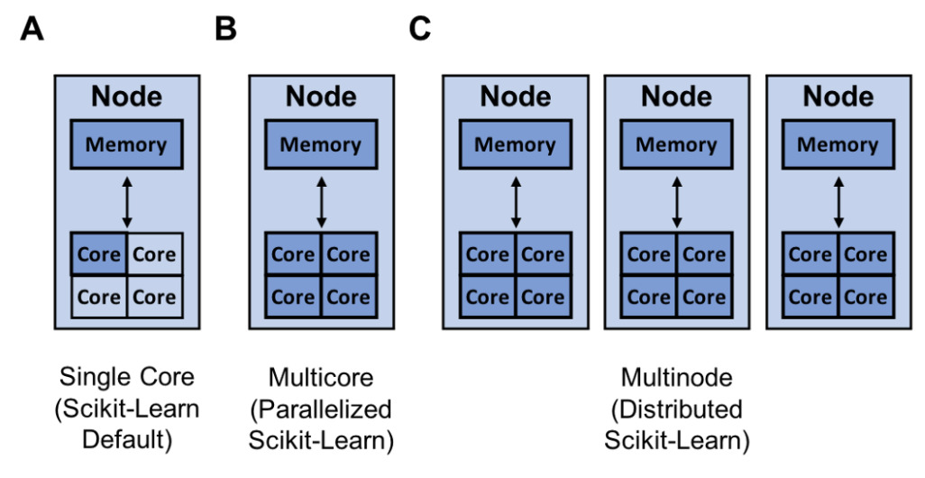
This post gives an overview of different ways to speed up your scikit-learn models and discusses some limitations of each approach.

Distill Archive 2021-01-30 20:00 UTC Score 10.0 AI-038-20210130-ai-specialis-0dc8e03e Full article

Curve Circuits

Reverse engineering the curve detection algorithm from InceptionV1 and reimplementing it from scratch.

Distill Archive 2021-01-27 20:00 UTC Score 10.0 AI-038-20210127-ai-specialis-0ede2f7c Full article

High-Low Frequency Detectors

A family of early-vision neurons reacting to directional transitions from high to low spatial frequency.

Are there constraints for the variance of predicted probability on calibrated models?
Cross Validated 2021-01-24 07:21 UTC Score 18.0 AI-113-20210124-social-media-afa476fc Full article

Are there constraints for the variance of predicted probability on calibrated models?

I'm sorry if the title is too vague. I'm not really sure of what I ask, this is a somewhat speculative question... The setting is that I'm using XGBoost in a binary classification problem (40% positive class) , and I want to get predicted probabilities, so after the model is trained, I train an isotonic calibrier. What I get is the following: The first model, before calibration, was good enough in terms of AUC, obtaining 0,82. The probabilities were not calibried at all. After calibration, the probabilities are well calibrated, but I plotted the histogram of predicted probability and I got this: So, after seeing this histogram, I began to think that the model was not very informative, or too conservative. I mean, let's imagine that we had all possible models with perfect calibration in front of us. Which one will be the best? And the worst? I think the worst will be the model that predicts the base rate for all instances, as this is the bare minimum that a non-informative but calibrated model can give. And the best will be the model with two peaks, on 0 and 1, a model that "knows" for certain the class of each instance. In between, the rest of models could be ordered in terms of how concentred is the histogram around the mean. I'm not sure of what I'm saying, so I ask just in case there is a theory that supports this intuitions: Is it true that, among calibrated models, the more "disperse" the better? For example, the model with the bigger variance the better? And if so, if…

Data Science Stack Exchange 2021-01-22 13:01 UTC Score 21.0 AI-111-20210122-social-media-08200684 Full article

TypeError: Expected sequence or array-like, got

I am training a CNN, it runs well but I get an error when I try to get precision_score , recall_score and the f1_score . Here is a snippet of my code; # The next step is to split training and testing data. For this we will use sklearn function train_test_split(). features_train, features_test, labels_train, labels_test = train_test_split(features, labels, test_size=.2) features_train.shape, features_test.shape, labels_train.shape, labels_test.shape ((180568, 2677356), (45143, 2677356), (180568,), (45143,)) features_train.shape[0], features_train.shape[1], labels_train.shape[0] (180568, 2677356, 180568) n_timesteps, n_features, n_outputs = features_train.shape[0], features_train.shape[1], labels_train.shape[0] X_train = np.zeros((180568, 82, 1)) y_train = np.zeros((180568, 82)) n_timesteps, n_features, n_outputs = X_train.shape[1], X_train.shape[2], y_train.shape[1] n_samples = 1000 X = np.random.uniform(0,1, (n_samples, n_timesteps, n_features)) y = pd.get_dummies(np.random.randint(0,n_outputs, n_samples)).values model = tf.keras.models.Sequential([ tf.keras.layers.Conv1D(input_shape=(n_timesteps, n_features), activation='relu', kernel_size=2, filters=32), tf.keras.layers.MaxPooling1D(strides=3), #tf.nn.local_response_normalization((1, 1, 1, 1), depth_radius=5, bias=1, alpha=1, beta=0.5, name=None), tf.keras.layers.LayerNormalization(axis=1), tf.keras.layers.Conv1D(input_shape=(n_timesteps, n_features), activation='relu', kernel_size=2, filters=64), tf.keras.layers.MaxPoolin…

Why are the p-values of this mixed effect model non-uniform when there is no effect (synthetic data)?
Cross Validated 2021-01-21 21:07 UTC Score 18.0 AI-113-20210121-social-media-1fe94bf1 Full article

Why are the p-values of this mixed effect model non-uniform when there is no effect (synthetic data)?

I've been looking into using mixed effect models for a project, and along the way wanted to experiment with how they'd work on synthetic data. However, I'm confused by the results — if I generate what I think is null data (e.g. no true difference between two inputs), the p-value for their difference is skewed towards higher significance than I would expect. I'm not sure if I'm making an incorrect assumption about how mixed effect models are supposed to work, or if I'm generating it incorrectly. Here's what I've been doing: I have two sets of inputs, each with N distinct groups, and M samples per group. To draw outputs, for both sets of inputs, I draw N values to represent each group's baseline effect, and then M values per group to represent the random variances. I then add those up for both sets of inputs, run a mixed effect model, and generate a p-value. I repeated this 1000 times and made a histogram of the p-values. Here's the code: import numpy as np import pandas as pd import statsmodels.api as sm import matplotlib.pyplot as plt num_groups = 10 num_samples_per_group = 20 num_iter = 1000 group_var = 1.0 random_var = 1.0 # Build basic dataframe w/ two inputs (input_0 and input_1), each with num_groups different groups, each # containing num_samples_per_group individual samples. df = pd.DataFrame({ 'input': ['input_0'] * num_samples_per_group * num_groups + ['input_1'] * num_samples_per_group * num_groups, 'group': ( ['input_0_group_%s' % (i % num_samples_per_group) for i…

Jay Alammar Blog 2021-01-19 00:00 UTC Score 33.0 USR-0113-20210119-ai-specialis-e1508f35 Full article

Finding the Words to Say: Hidden State Visualizations for Language Models

By visualizing the hidden state between a model's layers, we can get some clues as to the model's "thought process". Figure: Finding the words to say After a language model generates a sentence, we can visualize a view of how the model came by each word (column). Each row is a model layer. The value and color indicate the ranking of the output token at that layer. The darker the color, the higher the ranking. Layer 0 is at the top. Layer 47 is at the bottom. Model:GPT2-XL Part 2: Continuing the pursuit of making Transformer language models more transparent, this article showcases a collection of visualizations to uncover mechanics of language generation inside a pre-trained language model. These visualizations are all created using Ecco, the open-source package we're releasing In the first part of this series, Interfaces for Explaining Transformer Language Models, we showcased interactive interfaces for input saliency and neuron activations. In this article, we will focus on the hidden state as it evolves from model layer to the next. By looking at the hidden states produced by every transformer decoder block, we aim to gleam information about how a language model arrived at a specific output token. This method is explored by Voita et al.. Nostalgebraist presents compelling visual treatments showcasing the evolution of token rankings, logit scores, and softmax probabilities for the evolving hidden state through the various layers of the model.

Maximum likelihood observation with a constraint
Cross Validated 2021-01-17 13:01 UTC Score 12.0 AI-113-20210117-social-media-f9e63af0 Full article

Maximum likelihood observation with a constraint

I have a vector $\mathbf{x}$ of $n$ real random variables. The random variables can be assumed to follow a multivariate normal or log-normal distribution (assuming $\mathbf{x}>0$ is ok). I would like to analytically obtain the probability that the sum of the random variables decreases below a certain threshold, i.e. ${\mathbf{1}^T\mathbf{x}}\leq\sqrt{\mathbf{x}^T\mathbf{Q}\mathbf{x}}$ , where $\mathbf{1}$ is a vector $n$ ones and $\mathbf{Q}$ is a positive definite $n\times n$ real matrix. I cannot find the distribution of ${\mathbf{1}^T\mathbf{x}}-\sqrt{\mathbf{x}^T\mathbf{Q}\mathbf{x}}$ or ${\mathbf{1}^T\mathbf{x}}/\sqrt{\mathbf{x}^T\mathbf{Q}\mathbf{x}}$ . Therefore I have started to look for alternative ways to find the probability: Is there any sense to find the maximum likelihood observation s.t. the constraint and then obtain the probability from a cdf? For example, could I apply the normal log-likelihood as follows: $\arg\max$ $f(\mathbf{x} \mid \mathbf{\mu},\mathbf{\Sigma}) =\frac{1}{2} [\ln(|\mathbf{\Sigma}|) + n \ln\left (2\pi \right ) + (\mathbf{x}-\mathbf{\mu})^T\mathbf{\Sigma}^{-1}(\mathbf{x}-\mathbf{\mu})]$ subject to ${\mathbf{1}^T\mathbf{x}}-\sqrt{\mathbf{x}^T\mathbf{Q}\mathbf{x}} \leq 0$ . If this is nonsense please elaborate why.

Train autoencoder to reconstruct 2D Gaussian data
Cross Validated 2021-01-16 05:58 UTC Score 18.0 AI-113-20210116-social-media-d7b6dd31 Full article

Train autoencoder to reconstruct 2D Gaussian data

I am trying to train an autoencoder to reconstruct 2D Gaussian data. These datapoints are simply sampled from Gaussians with means and covariances chosen randomly. An illustration of what I am trying to do can be visualized below for datapoints from 3 different Gaussians The blue crosses are the training data and the orange points are the reconstruction of the autoencoder. The goal is to have the orange points match as closely as possible to the blue points. I am using MSE loss for now, although KL divergence between the input and output distributions seem to make more sense, but is trickier to implement for backprop. For each training set I sample 100 2D coordinates from a different Gaussian, say (x,y) and I stack them into a 200-long feature vector [x1, y1, x2, y2, ... , x100, y100] and pass in mini-batches of these into the autoencoder. I sort these points by the L2 norm of the tuples (x,y), which I've found to help a bit. I've tried basic fully connected autoencoders (200 input/output neurons) and also convolutional autoencoders. Any tips on how I could make it work better? Thanks!

Is it ok to use volunteers for prospective cohort studies
Cross Validated 2021-01-15 03:07 UTC Score 12.0 AI-113-20210115-social-media-6681c7ee Full article

Is it ok to use volunteers for prospective cohort studies

Prospective cohorts are ones where the exposure is known but not the disease outcome. Volunteer bias is where volunteers tend to be healthier. I've been told because of this volunteer bias, we should not use volunteers for our epidemiology experiments. I can see why this is true in the case of prevalence studies. Volunteers tend to smoke less and thus we will underestimate the prevalence of smoking if we only get volunteers. But I don't see why this must be true for prospective cohort studies. Let's say there's been a nuclear accident and we rush to attract volunteers from those who've been exposed to radiation. All my volunteers, exposed and unexposed, are very fit and don't smoke. Their general better health could mean they recover better from radiation. One could say this skews results. However, given that my other unexposed volunteers are equally healthy - wouldn't this be a fair comparison? Is there still volunteer bias here?

How to extract parameters from a text using AI/NLP
AI Stack Exchange 2021-01-13 13:34 UTC Score 23.0 AI-110-20210113-social-media-8c81b4b2 Full article

How to extract parameters from a text using AI/NLP

lets say I have three texts: "make a heading that says hello word" "make a heading of hello world" "create heading consist of hello world" How can I fetch those groups of words using AI which is referring to heading i.e hello world in this case. Which AI frameworks or libraries can do that? in all examples heading is pointing to hello world (which i am referring as group of words). so basically i want those words which will be a part of heading or in other word there is a relationship between them. another example i can give is "I am watching Breaking bad" so there is a relationship between watching and breaking bad and i want to extract what are you watching. What's the best approach? Do I have to train a model for that or there are some other techniques that can get it done?

VAR model variable selection
Cross Validated 2021-01-11 21:06 UTC Score 16.0 AI-113-20210111-social-media-e55e7f3e Full article

VAR model variable selection

I'm required to use two time series models in my exam project. I want to use a stock price of an energy company, and then explain it first using ARIMA, and then adding other variables and using VAR. My problem is that I can't find variables which pass the Granger test of causality. I have tried prices of commodities, competitor stock prices, etc. So now I have opted to use two of the same company's stocks, but just listed on different stock exchanges (same company, same currency - one stock trading in Germany, the other in Brussels) Obviously, the stock on both markets is impacted by the same unobserved variables. Is this a huge mistake, or can I proceed if I discuss and show that I am aware of omitted variable bias?

Data Science Stack Exchange 2021-01-11 06:25 UTC Score 12.0 AI-111-20210111-social-media-b6b9df2d Full article

Time series forecasting with constraints

I want to predict the passenger flow volume of an airline route, which subjects to supply capacity constraints of the route (i.e., the passenger flow volume should not be higher than the supply capacity). Are there any algorithms that could be used to do this kind of forecasting problem with constraints?

Quasi-random sequence with discrete variables with differing number of levels
Cross Validated 2021-01-08 19:01 UTC Score 12.0 AI-113-20210108-social-media-4cc878b0 Full article

Quasi-random sequence with discrete variables with differing number of levels

My question is probably worded incorrectly but here it is: I have (say) 3 discrete random variables: x1: has 15 levels (uniform pdf for simplicity) x2: has 3 levels (uniforms) x3: has 4 levels (uniform) I want to generate n samples in such a way that: there are no repetitions of samples as n --> 15x3x4 the entire "full factorial" sample is generated; When generating (n+d) set of samples, the first n samples are the identical for any d I tried to use Sobol quasi random sequence to generate this sample BUT I am not able to satisfy #1 above without retaining all prior points in memory and checking for duplicates. This is something I would like to avoid. Thanks for your answers.

Alignment Newsletter 2021-01-04 01:32 UTC Score 35.0 USR-0153-20210104-ai-specialis-4e07dab9 Full article

FAQ: Advice for AI alignment researchers

Consider reading How to pursue a career in technical AI alignment. It covers more topics and has more details, and I endorse most if not all of the advice. To quote Andrew Critch: I get a lot of emails from folks with strong math backgrounds (mostly, PhD students in math at top schools) who are […]

Prove the linear transformation of Gaussian distribution from Bayesian perspective
Cross Validated 2020-12-24 07:31 UTC Score 12.0 AI-113-20201224-social-media-974e2d3b Full article

Prove the linear transformation of Gaussian distribution from Bayesian perspective

I understand the linear transformation property of Gaussian distribution, i.e., if $x\sim\mathcal{N}(\mu, \sigma^2)$ , then $cx\sim\mathcal{N}(c\mu, c^2\sigma^2)$ given $c$ is a constant. If we write this as a marginalization: $$p(f(c)|c) = \int p(f(c)|c, x)p(x)dx$$ and here $f(c) = cx$ . $p(x)$ can be expressed as $\dfrac{1}{\sqrt{2\pi}\sigma}e^{-\frac{1}{2\sigma^2}(x-\mu)^2}$ . But how do we obtain $p(f(c)|c)$ from the above marginalization form (or the posterior predictive distribution, here I simplified the posterior to just $p(x)$ ), that is to get $$\quad \, p(f(c)|c) = \dfrac{1}{\sqrt{2\pi}c\sigma}e^{-\frac{1}{2c^2\sigma^2}(f(c)-\mu c)^2} \quad\text{?}$$ What troubles me is $p(f(c)|c, x)$ . I think it is $1$ , as it is deterministic when $c$ and $x$ are given, but I'm not sure how to proceed.

Cross Validated 2020-12-23 19:04 UTC Score 13.0 AI-113-20201223-social-media-c7b5a160

MSE of correlations

These might be dumb questions but I am having trouble to wrap my head around of a particular problem. I have a sparse count matrix $G $ that I want to optimize which is $N \times p$ . Also, I have correlation matrix $C_{ij}$ which is $N \times N$ that I want matrix $G$ to be optimized for. So, without any constraints I have the following loss function: $$ \text{loss} = \sum_i\sum_j (\operatorname{corr}(G_i, G_j) - C_{ij})^2 $$ where $G_i$ is a vector $1 \times p$ and $i = j = 1,\ldots,N$ . So, my first question is how can I solve/implement this particular problem ? My second question is related to my lack of knowledge regarding defining optimization problems :) First of all, as I mentioned above $G$ is a count matrix and it is very sparse and I also want to keep the distribution of each $G_i$ while optimizing, not just randomly change it as it is described above because the initial values are important. So, my question is that is there a way for me to add these information into the problem design ?

Choice of Smoothing Kernel in ABC
Cross Validated 2020-12-23 11:40 UTC Score 18.0 AI-113-20201223-social-media-1cae7345 Full article

Choice of Smoothing Kernel in ABC

In Approximate Bayesian Computation, one approximates an intractable likelihood by convolving it with some smoothing kernel $K$ as \begin{align} \ell^{\text{ABC}} ( x | \theta ) = \int \ell ( z | \theta ) \, K (x, z) \, dz. \end{align} Common choices for $K$ include $K(x, z) = \mathbf{I} \left[ d(x, z) \leqslant \varepsilon \right]$ and $K(x, z) = \exp \left( - \frac{d (x, z)^2 }{2 \varepsilon^2 }\right)$ , where $d$ is some sort of distance-like function, and $\varepsilon$ is some 'tolerance / threshold' parameter. My question is: in practice, what guides the choice of $K$ ? For example, which features of a problem should encourage a user to prefer a uniform kernel to a Gaussian kernel? Ignore the choice of summary statistics, threshold parameter, and so on. I am aware of the 'model error' perspective of R. Wilkinson (as in this paper ), which is very useful in some circumstances. Have alternative perspectives arisen in the interim? e.g. are there purely algorithmic reasons to prefer a specific kernel?

Jay Alammar Blog 2020-12-17 00:00 UTC Score 39.0 USR-0113-20201217-ai-specialis-fb351fb3 Full article

Interfaces for Explaining Transformer Language Models

Interfaces for exploring transformer language models by looking at input saliency and neuron activation. Explorable #1: Input saliency of a list of countries generated by a language model Tap or hover over the output tokens: Explorable #2: Neuron activation analysis reveals four groups of neurons, each is associated with generating a certain type of token Tap or hover over the sparklines on the left to isolate a certain factor: The Transformer architecture has been powering a number of the recent advances in NLP. A breakdown of this architecture is provided here . Pre-trained language models based on the architecture, in both its auto-regressive (models that use their own output as input to next time-steps and that process tokens from left-to-right, like GPT2) and denoising (models trained by corrupting/masking the input and that process tokens bidirectionally, like BERT) variants continue to push the envelope in various tasks in NLP and, more recently, in computer vision. Our understanding of why these models work so well, however, still lags behind these developments. This exposition series continues the pursuit to interpret and visualize the inner-workings of transformer-based language models. We illustrate how some key interpretability methods apply to transformer-based language models. This article focuses on auto-regressive models, but these methods are applicable to other architectures and tasks as well. This is the first article in the series. In it, we present explo…

Accuracy is 100% but model.predict is totally wrong! what could be the problem? (Autoencoder NN) [closed]
Cross Validated 2020-12-12 20:09 UTC Score 26.0 AI-113-20201212-social-media-cb7b55bc Full article

Accuracy is 100% but model.predict is totally wrong! what could be the problem? (Autoencoder NN) [closed]

I have an Autoencoder model that receives 4 different vectors { (1,0,0,0) , (0,1,0,0) , (0,0,1,0) , (0,0,0,1) } The encoder transforms the vectors to vectors size 2, which get inside an "NLPN channel" which is a channel with nonlinear phase noise, and then goes to the decoder that reconstructs the original vector. Architecture: 4->50->2->NLPN->2->50->4 (Softmax) The loss function is mse between the input, and the input ( self.model.fit(self.x, self.x) ) The code is pretty basic: the first cell is just some simple functions defined, then it's the autoencoder class, then it's the training, and then it's the prediction which shows that for each vector 1,0,0,0 and so on, the decoder predicts (~0.25,~0.25,~0.25,~0.25) which shows that the NN has no idea what it's doing. CODE: https://colab.research.google.com/drive/1nFymmEloUSa1yjS7e5CPGsKwqP1HjS57?usp=sharing

Statsmodels Linear Regression with ARIMA errors model not including the ARIMA error in prediction?
Cross Validated 2020-12-09 16:55 UTC Score 23.0 AI-113-20201209-social-media-7cbce1bb Full article

Statsmodels Linear Regression with ARIMA errors model not including the ARIMA error in prediction?

I have fit a SARIMAX (1, 0, 0) model to a timeseries dataset consisting of 1 endogenous timeseries ("Y") and 1 exogenous timeseries ("X"). My exogenous timeseries in the model was defined with sm.add_constant. Stationarity and invertibility were enforced in the Statsmodels SARIMAX model. trend = 'n' The model parameters were: const = -0.0218685769848199 X = 1.02191782244191 ar.L1 = 0.780715685830694 sigma2 = 4.942018879444325E-06 I generated the predictions (including out of sample forecasts) using predicted_mean. For the last (oldest) observed record in the timeseries: the model's predicted (and last fitted) value is 0.9948866129977041 the Y value is 1.00547070891269 the X value is 0.994948094292246 the residual (.resid) is 0.010584096 For the first prediction: the model's predicted value is 0.990566738090985 the X value is 0.990720870937109 (There is no Y value, and also no residual) In trying to manually recreate the forecasts in Excel, I was only able to match the Statsmodels forecast when I don't include the ARIMA-modelled residuals in my calculation. I was able to match the provided residual. Here's the model I followed: ϵ^t−1 = yt−1 − (β0 + β1xt−1) = 0.010584096 (matches the Statsmodels residual for the last (oldest) observed record) ϵt = ϕ(ϵt−1) = 0.00826316972 Now we can compute yt which should be: yt = β0 + β1xt + ϵt = -0.0218685769848199 + (1.02191782244191 * 0.990720870937109) + 0.00826316972 = 0.99882990780828 (which doesn't match the Statsmodels prediction valu…

How to match regions in difference-in-differences analysis
Cross Validated 2020-12-04 02:39 UTC Score 9.0 AI-113-20201204-social-media-02a6b804 Full article

How to match regions in difference-in-differences analysis

I've had an idea for a project to work on over winter break. It involves a difference-in-differenced analysis of two similar-sized cities on different sides of a state border. How do I confirm that the two cities are similar enough in their characteristics? Is it an eye test or is there a statistical methodology? I would also appreciate any suggested readings.

Extracting the fitted expected number of points from mppm in spatstat (in R)
Cross Validated 2020-12-02 23:52 UTC Score 12.0 AI-113-20201202-social-media-c3b00510 Full article

Extracting the fitted expected number of points from mppm in spatstat (in R)

When fitting a Poisson process model on multiple point patters using the spatstat R package (mppm function), is there a computationally efficient way to extract the fitted expected number of points from the mppm fit? I expand with a toy example below: Let's say that my data are point patterns over T time periods and I have a single spatio-temporal predictor in the form of an image (spatstat im class). I generate such toy data here: set.seed(1234) library(spatstat) # Number of time periods. For each time period I observe a point pattern. time_points Then, we can use mppm to fit a poisson process model for the point pattern data on the predictor. We can do so with the following code: mod_dta In order to extract the estimated conditional intensity function we can use the predict.mppm function: mod_dta$fitted_cif which we can use to extract the expected number of points for each time period as the integral of the conditional intensity function: plot(with(mod_dta, integral(fitted_cif))) However, this process can be slow if the number of time periods time_points is large, and the value for ngrid in predict.mppm is set to large (to improve accuracy). I wonder if the fitted expected number of points can be extracted directly from the mppm fit ( pp_mod in the example) without having to define the conditional intensity as an image and integrate over it. Thank you for your help.

Determining coin mint year from a known sample based on elemental composition
Cross Validated 2020-12-02 11:33 UTC Score 17.0 AI-113-20201202-social-media-96f1e73a Full article

Determining coin mint year from a known sample based on elemental composition

I have data on the metallic compositions (percentages of specific elements) of 30 coins, each minted in a different year from 1902 to 1967. I also have the composition of a coin minted in an unknown year which I would like to try and classify to a year of minting through comparison with the reference dataset. How would I go about doing this? I attempted discriminant analysis in SPSS using Coin Year (numeric; nominal) as the grouping variable and the percentages of each metal element (Cu, Sn, Zn, Pb, As, Zr, Ni, Nb, Co, W, Mn, Se) as the Independents, but received the error: “Warnings: There are 31 non-empty groups and 31.000 (31 unweighted) cases that are valid. Not enough weighted or unweighted cases. Execution of this command stops.” I suspect this is because there is only one set of values associated with each year, but I’m stuck on how to overcome this. I thought about potentially using a Euclidean distance measure, but I’m not sure. Any advice?

Measure of distance between two survey responses
Cross Validated 2020-12-01 16:44 UTC Score 9.0 AI-113-20201201-social-media-5818c691 Full article

Measure of distance between two survey responses

I've found some survey data where respondents answer 63 question by giving a response for each question between 0-10 (0 for strong disagreement, 10 for strong agreement). So I can view every respondent as a integer point in $[0,10]^{63}$ . Question: is there a "standard" way to measure the distance between two respondents? Something like the taxicab distance between them seems somewhat reasonable, but likewise so does any $L^p$ -distance. Though these wouldn't account for questions that contributed the most of least variation in responses, for example. My intended application is using this to measure distances between points to experiment with persistent homology.

Using Monte Carlo standard error to determine the ideal number of trials?
Cross Validated 2020-12-01 00:27 UTC Score 12.0 AI-113-20201201-social-media-6b28a823 Full article

Using Monte Carlo standard error to determine the ideal number of trials?

I am doing a simulation study that involves estimating the parameter $\theta$ under a specific experimental design. $\theta$ is the parameter that take on the value 1 if algorithm A is better than algorithm B, and 0 otherwise. I am repeating my simulation study for $N$ times so that I can count the number of times where the algorithm A performed better than the algorithm B. If the number of times that algorithm A performed better than algorithm B is greater than $\frac{N}{2}$ , then I can conclude that $\theta$ is likely to be equal to 1. But I am not sure how to pick the "right" value for $N$ , and someone advise me that I can analyze the Monte Carlo standard error of the probability to determine the value for $N$ . However, I am not very familiar with doing this kind of thing, and I am seeking a guidance on this. The only idea that I can come up with is that if we let $\hat{\theta}$ to be an indicator variable that is equal to 1 if the event occurs, then $\sqrt{\frac{1}{N(N-1)}\sum^{N}_{i=1}(\hat{\theta}_i-\bar{\theta})^2}$ can be used as the Monte Carlo SE of estimate of bias for $\theta$ , where $\bar{\theta}$ is the sample average of $\hat{\theta}$ 's. However, I am not exactly sure how to use this information to determine the optimal value for $N$ . Should I just try varying the value of $N$ and collect $\theta_1 \cdots \theta_N$ from each value of $N$ , calculate the Monte Carlo SE for each case, and see if which value of $N$ would minimize Monte Carlo SE? How can I d…