Latest AI/ML News
28097 matching items

"repeated measures ANOVA" vs "ANOVA with subject as random effect" vs "repeated measures ANOVA with subject as random effect"
What is the difference between running a repeated measures ANOVA (the measure is repeated across time for each subject) vs an ANOVA with a subject as a random effect?` I have also seen mention of a "repeated measures ANOVA with subject as random effect". For context I have 6 groups and 3 post-baseline time points per group/subject. Each subject is a member of one group. I would like to compare means of both different groups at the same time point (ex group 1 vs group 3 at time point B) and means of the same group at different time points (ex. group 1 at time point B vs group 1 at time point C). I will use ls-means to compare means, but I don't really understand the differences between the above three model categories. If there even is a difference! Thank you very much!
AI companies are pivoting from creating gods to building products. Good.
Turning models into products runs into five challenges
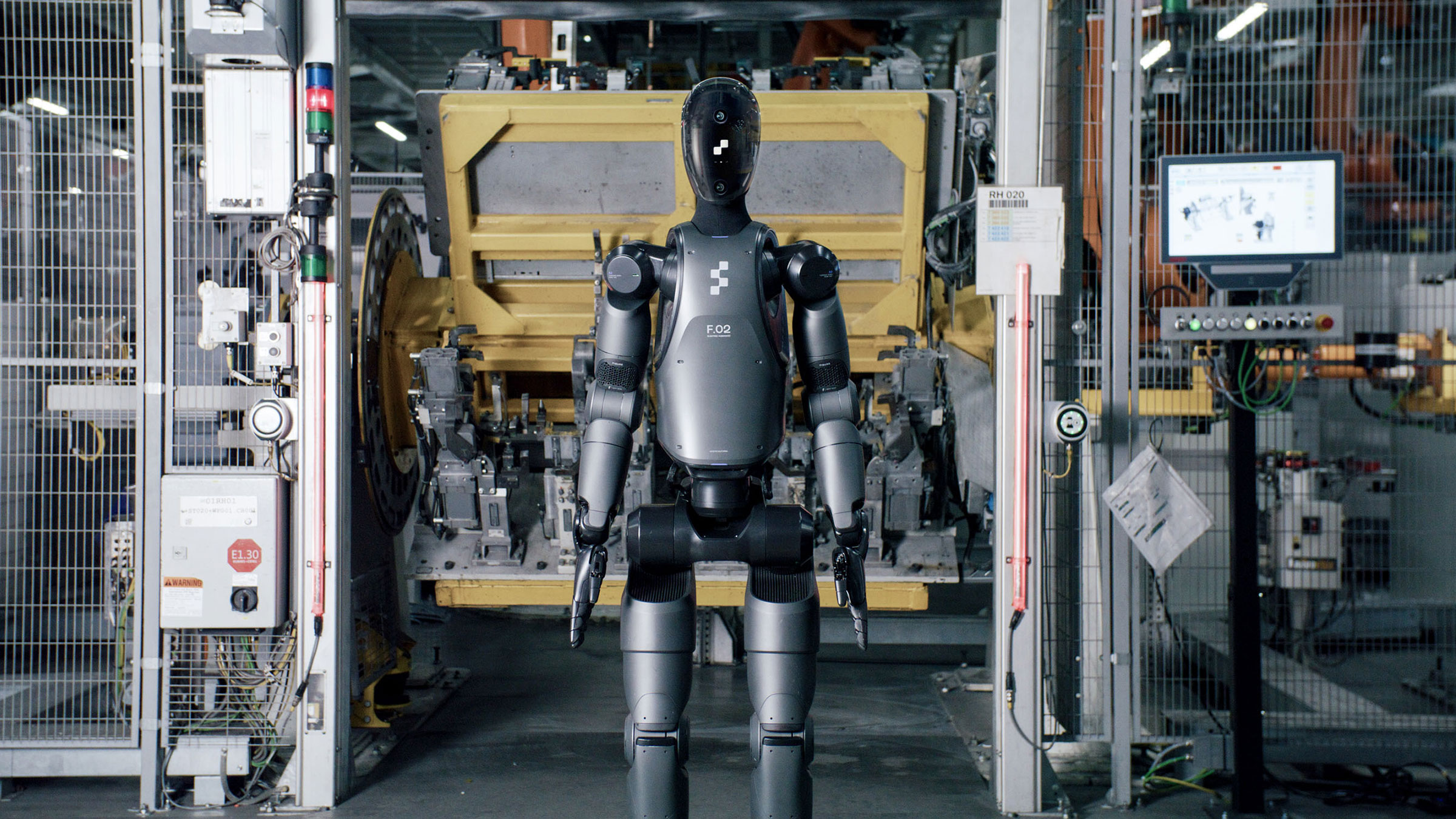
Humanoid Robots on the Rise: Industry Advances, Key Players, and Adoption Timelines
The robotics industry stands on the brink of a significant transformation, with many experts – including NVIDIA CEO Jensen Huang – suggesting that we might be approaching a "ChatGPT moment" for robotics. The post Humanoid Robots on the Rise: Industry Advances, Key Players, and Adoption Timelines appeared first on TOPBOTS .
Utilizing Symbolic Regression to discover a larger class of splits for Decision Trees
This work is based on the paper: K.S. Fong and M. Motani, “Symbolic Regression Enhanced...
Any relation between two KL divergences?
I am using a KL divergence to measure the difference between distributions, but I would like to compare the results to each one another, because the probability distributions I'm measuring are correlated. What is a good measure for comparing two KL divergences on related distributions? Ex. If I'm looking at some characterization data for a test, let's say X-ray diffraction patterns for a metal sample. I get an XRD pattern of intensity vs. diffraction angle, and can create a probability distribution for that in a reference state (room temp, new sample). I then run the same XRD test on the same sample while I vary temperature, and for that temperature I get a new distribution of my XRD data, and I can calculate the KL divergence for that distribution relative to my reference one. Let's say I then cold-roll my metal sample, and run the same XRD experiment, and then calculate the KL divergence with the same reference state for those distributions. I have two KL divergence results, and I know that there are variables for the metal sample, temperature vs. strength, that are correlated. Is there any comparison technique between divergences to tell me how much one distribution diverged relative to another? Especially if the variables are interrelated? Edit: Changing the example to be more specific.
Lower bound of KL divergence of Gaussian mixture with Gaussian (univariate)
I'm interested in a non-zero Kullback-Leibler divergence lower bound between a Gaussian mixture $q$ and a standard Gaussian $p(x) = \mathcal N(x \mid 0,1)$ , both univariate : $D_{KL}(q \parallel p)$ . I'm aware of this question , but I conjecture that with some constraints the problem might become easier. My constraints: The Gaussian mixture is guaranteed to have mean zero The Gaussian mixture is guaranteed to have variance lower bounded by $\gamma^2$ . I skim over Hershey & Olsen (2007) , which mentions a pretty trivial Gaussian approximation of the KL divergence in Section 4, where $q$ is approximated by a Gaussian $\bar q(x) = \mathcal N(x \mid \mu, \sigma^2)$ , (here, $\mu \triangleq \mathbb E_q[x] = 0, \sigma^2 \triangleq \mathbb E_q[x^2] - \mathbb E_q[x]^2 \ge \gamma^2$ ); and then the target KL is approximated by $D_{KL}(\bar q \parallel p)$ . However, the paper says this is a poor approximation, and does not mention whether it's a bound either. In Melbourne et al. (2018) , the authors propose an upper bound on the entropy of a mixture distribution. Since $D_{KL}(q \parallel p) = -\mathbb H(q) - \mathbb E_q[\log p(x)]$ , I'm able to take advantage of it, provided that I know how to upper bound the expected log density term , which is outside my expertise again.
Bayesian hierarchical model for comparing reviewers
I am working on a research paper about reviewing people's expertise. I have 21 respondents, each answered 10 questions. Now I have asked 4 groups of reviewers (each group consists of 3 people) to grade the answers between 1 and 5 (5 best). I have used Fleiss' Kappa to measure inter-rater reliability between reviewers in the same group. Unfortunately one reviewer asked me to include a Bayesian hierarchical model to account for the variability among raters and to provide a probabilistic measure of rater consistency. This would allow for a more nuanced understanding of rater behavior and the inherent uncertainties in human judgment, which are oversimplified by the use of a linear scale in the current methodology. In my opinion it is an over-complication. I wanted to check whether people from different backgrounds can assess people in the same topic. I do not see any benefits from using Bayesian hierarchical model for comparing reviewers. I am trying to perform this test, but nonetheless I would like to respond to the reviewer POLITELY that this is not a use-case for this model and Fleiss kappa is sufficient. Could you help me, or prove me wrong?
AI in Finance Global Challenge Startup Grant Awardee
In June 2023, the Monetary Authority of Singapore (MAS) launched the 8th edition...
Mechanistic Anomaly Detection Research Update
Interim report on ongoing work on mechanistic anomaly detection

We Need Positive Visions for AI Grounded in Wellbeing
Introduction Imagine yourself a decade ago, jumping directly into the present shock of conversing naturally with an encyclopedic AI that crafts images, writes code, and debates philosophy. Won’t this technology almost certainly transform society — and hasn’t AI’s impact on us so far been
Leveraging Generative AI in Project Management
Introduction The project management landscape is undergoing a transformative shift, driven by the rapid advancements...
Open Source Automated Interpretability for Sparse Autoencoder Features
Building and evaluating an open-source pipeline for auto-interpretability
Learning to Generate Unbounded 3D Scenes from Image Collections
Introduction Scene generation has raised considerable attention in recent years, addressing the growing need...

Accelerate Your AI Skills: Essential Generative AI Courses for Developers
Generative AI is a rapidly evolving field with a plethora of fascinating applications, from creating realistic images and videos to generating human-like text and beyond. As the technology advances, the demand for skilled professionals who can harness the power of generative AI is growing exponentially. However, navigating the myriad of tutorials and courses available can […] The post Accelerate Your AI Skills: Essential Generative AI Courses for Developers appeared first on TOPBOTS .
Congratulations to Stanford AI Lab PhD student Dora Zhao for an ICML 2024 Best Paper Award!
Congratulations to Stanford AI Lab PhD student Dora Zhao for an ICML 2024 Best Paper Award for a paper from her work at Sony AI on: Measure Dataset Diversity, Don’t Just Claim It
Congratulations to Aaron Lou, Chenlin Meng, and Stefano Ermon for an ICML 2024 Best Paper Award!
Congratulations to Aaron Lou, Chenlin Meng, and Stefano Ermon for an ICML 2024 Best Paper Award: Discrete Diffusion Modeling by Estimating the Ratios of the Data Distribution
Congratulations to Marco Pavone for a Robotics: Science and Systems Conference Best Paper Award!
Congratulations to Marco Pavone for winning the best paper award at the Robotics: Science and Systems Conference on AI Safety for autonomous systems.
AI existential risk probabilities are too unreliable to inform policy
How speculation gets laundered through pseudo-quantification
Building A Generative AI Platform
After studying how companies deploy generative AI applications, I noticed many similarities in their platforms. This post outlines the common components of a generative AI platform, what they do, and how they are implemented. I try my best to keep the architecture general, but certain applications might deviate. This is what the overall architecture looks like. This is a pretty complex system. This post will start from the simplest architecture and progressively add more components. In its simplest form, your application receives a query and sends it to the model. The model generates a response, which is returned to the user. There are no guardrails, no augmented context, and no optimization. The Model API box refers to both third-party APIs (e.g., OpenAI, Google, Anthropic) and self-hosted APIs. From this, you can add more components as needs arise. The order discussed in this post is common, though you don’t need to follow the exact same order. A component can be skipped if your system works well without it. Evaluation is necessary at every step of the development process. Enhance context input into a model by giving the model access to external data sources and tools for information gathering. Put in guardrails to protect your system and your users. Add model router and gateway to support complex pipelines and add more security. Optimize for latency and costs with cache. Add complex logic and write actions to maximize your system’s capabilities. Observability, which allow…
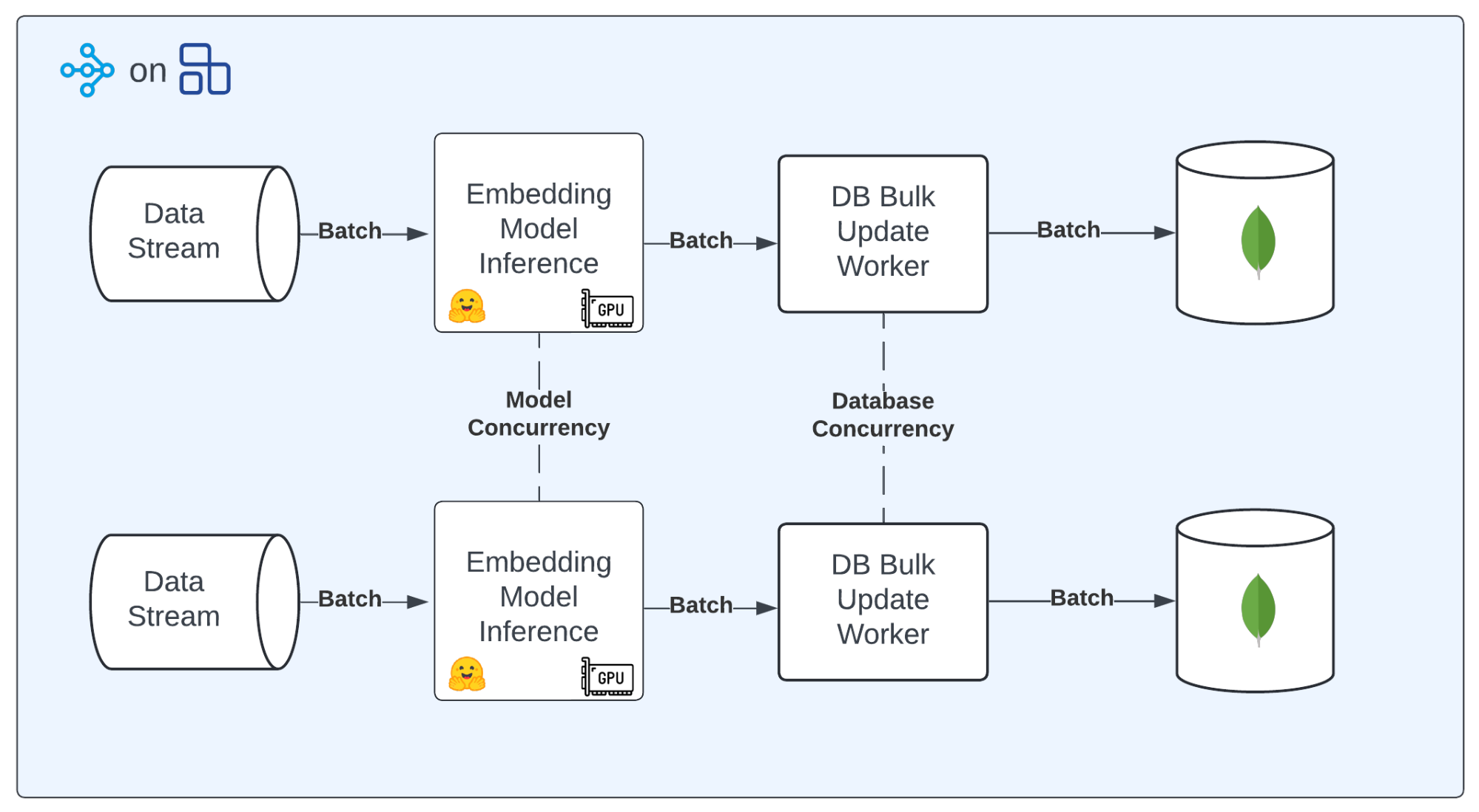
Writing Kullback–Leibler divergence in terms of the score function
Assume we have two density functions $p(x)$ and $p'(x)$ for $x\in R^d$ . I would find a connection between Kullback–Leibler divergence between two densities in terms of the difference between the gradient of the log densities: $\nabla_{x} \log p(x)$ and $\nabla_{x} \log p'(x)$ . Something like $$\int p(x)\log\frac{p(x)}{p'(x)}dx\le \frac{1}{2}E_{x}||\nabla_{x} \log p(x)-\nabla_{x} \log p'(x)||_2^2.$$ Can anyone help me please. I have already tried starting the definition of the KL and then integrating by part, but I stuck at some points then.
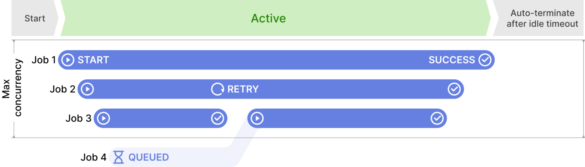
Fair comparison method for a biased physics-based model and its ML-correction version
I'm working with two prediction models: A calibrated physics-based model that consistently overestimates and has a fixed bias. An XGBoost model that predicts the error of the physics model to create corrected predictions. (The dataset contains the physics model's predictions and the target variable. We then predict the error between the target variable and the physical models prediction) I'm trying to fairly compare these models, but I'm unsure about the best approach. Simply using MAPE for both doesn't seem meaningful due to the known bias in the physics model. Here's what I'm considering: For the physics model: Calculate errors: errors = physics_model_prediction - actual_value Compute mean error: mean_error = errors.mean() Adjust errors: adjusted_errors = errors - mean_error Calculate MAPE: MAPE(adjusted_errors, actual_value) For the corrected model: Calculate MAPE(corrected_prediction, actual_value) Is this approach valid? The residuals' distribution in the correction model is slightly skewed but close to normal, tending to overestimate at certain values. But I'm wondering if this method is statistically sound. If there are better ways to compare the improvements I would appreciate any insights!
Why using mutual information is allowed for feature selection if depends on the "scale" of entropies?
It is common to use mutual information as feature selection method. However, I fail to see why this is the case, since the mutual information $I(X, Y)$ depends on both entropies $H(X)$ and $H(Y)$ via the formula : $$ I(X, Y) = H(X) + H(Y) - H(X,Y)$$ meaning that comparing $I(X_i, Y)$ and $(X_j, Y)$ as a measure for selecting between $X_i$ and $X_j$ is not straightforward since the measure can be bloated by the marginal entropies. It is like selecting between $X_i$ and $X_j$ based on the covariance with $Y$ instead of correlation. The only way I can think that such a comparison is allowed is due to the equivalent formula: $$I(X, Y) = H(Y) - H(Y|X)$$ As the first term $H(Y)$ is the same for all $X_i$ then the ramking shouldn't depend on the "scale" of $H(Y)$ . Is that correct or am I missing something?

Making Insights-Driven Decisions in an Ecosystem of Ecosystems
Our approach to securing our cloud environments
Les sciences du numérique à la conquête du ciel et de l’espace
Les sciences du numérique à la conquête du ciel et de l’espace mtestari mar, 07/09/2024 - 15:23 Après le lancement réussi d’Ariane 6 en juillet 2024 à Kourou, et alors que le nombre de voyageurs aériens atteint de nouveaux records en 2025, les sciences et technologies du numérique revêtent désormais une importance cruciale dans les domaines de l’aérospatial et l’aéronautique. © Pixabay/ Photo V. Stefanov Ces deux secteurs, très présents en Nouvelle-Aquitaine et en Occitanie, couvrent également des enjeux sociétaux et économiques significatifs. C’est tout un écosystème, opéré par Aerospace Valley , premier pôle de compétitivité européen, qui participe à l’étude, la conception, la fabrication et la commercialisation de ces technologies. Dans ce contexte, les équipes du Centre Inria de l’université de Bordeaux offrent à leurs partenaires industriels et académiques, les outils et les connaissances nécessaires pour renforcer la sécurité, la compétitivité et la décarbonation des systèmes, en s’appuyant sur leurs expertises telles que la modélisation, la simulation et la cryptographie . La conception des systèmes aéronautiques : un challenge scientifique pour chaque composante Il est primordial de développer des produits (aéronefs, avions, drones, lanceurs de satellites) les plus performants possible d’un point de vue du service rendu que de l’optimisation de la ressource exploitée. Grâce à la modélisation et à la simulation, Inria contribue à la création de modèles précis et réali…
Using conditional probability as an estimate in a loss function
I have a rather large ML framework that takes multiple conditional probability terms that are computed via classifiers/neural networks. This arbitrary loss function is computed via a function: loss_value = arbitrary_loss(probability1, probability2, ..., P(Y|Z)) I wish to have an end-to-end framework that computes everything and trains everything together. So I do not want to have an independently trained classifier. Say at some point I develop some intermediate values (embeddings) Z from the input samples X. I wish to model the conditional probability P(Y|Z) via an MLP softmax layer. This term P(Y|Z) is then estimated and plugged into the final loss which is the sum and product of other probabilities. P(Y|Z) = MLP(input_Z) #probability given input Z over labels My issue is that if I simply take the value of the softmax layer to estimate this probability and plug it in, at no point are the true labels taken into account for a supervised machine learning problem. How can I fix this without modifying the final loss function? TLDR: I need a probability term P(Y|Z) modeled via an MLP softmax layer to be used in a complex arbitrary loss function. How do i ensure this term is accurate via the true label values, so that it can be used in the final loss?
Understanding Empirical Bayes
I am trying to understand the basics of empirical bayes. I found myself struggling a lot to understand this so I tried to create a toy example involving the estimation of the success probabilities for a coin. 1) Traditional Bayesian Analysis (Beta-Binomial Conjugacy): Consider a sequence of $n$ coin tosses where we observe $X$ heads. The likelihood of observing $X$ heads given the true probability of heads $\theta$ is binomial: $$ P(X|\theta) = \binom{n}{X} \theta^X (1-\theta)^{n-X} $$ Chose a Beta prior distribution for the probability of heads $\theta$ : $$ P(\theta) = \text{Beta}(\alpha, \beta) = \frac{\theta^{\alpha-1} (1-\theta)^{\beta-1}}{B(\alpha, \beta)} $$ Using Bayes' theorem, the posterior distribution is proportional to the likelihood times the prior: $$ P(\theta|X) \propto P(X|\theta) P(\theta) $$ Substituting the binomial likelihood and the Beta prior, we get: $$ P(\theta|X) \propto \theta^X (1-\theta)^{n-X} \cdot \theta^{\alpha-1} (1-\theta)^{\beta-1} $$ $$ P(\theta|X) \propto \theta^{X+\alpha-1} (1-\theta)^{n-X+\beta-1} $$ Thus, the posterior distribution is also a Beta distribution: $$ P(\theta|X) = \text{Beta}(X + \alpha, n - X + \beta) $$ 2) Empirical Bayes: It seems like in Empirical Bayes, the parameters of the priors are estimated from the data instead of being chosen before hand. To me it makes more sense to use Method of Moments (instead of MLE) to estimate the parameters $\alpha$ and $\beta$ of the Beta prior. The sample mean $\hat{\theta}$ and sampl…
What's the relation between Generalized Policy Iteration (GPI), Actor-Critic, and Q-learning methods?
It seems to me that Generalized Policy Iteration (GPI) and Actor-Critic are the same, and Q-learning methods are a separate family of algorithms. I think both GPI and Actor-Critic describe the iterative process of policy evaluation (critic) and policy improvement (actor), while Q-learning is only bootstrapping using the Bellman optimality equation. To elaborate on my understanding: Policy evaluation (critic) is done via Monte-Carlo or temporal difference methods, including function approximation if necessary, and policy improvement (actor) can be done by being greedy (tabular case) or using the policy gradient theorem (large state space). Q-learning is not doing any of these. It's just trying to estimate the $Q^\ast$ using the Bellman optimality equation by iteratively fitting the Bellman optimality equation for Q value. I would appreciate it if anyone can confirm whether my understanding is correct or give a more systematic/precise summary of the taxonomy of online RL algorithms.
Extrinsic Hallucinations in LLMs
Hallucination in large language models usually refers to the model generating unfaithful, fabricated, inconsistent, or nonsensical content. As a term, hallucination has been somewhat generalized to cases when the model makes mistakes. Here, I would like to narrow down the problem of hallucination to cases where the model output is fabricated and not grounded by either the provided context or world knowledge. There are two types of hallucination: In-context hallucination: The model output should be consistent with the source content in context. Extrinsic hallucination: The model output should be grounded by the pre-training dataset. However, given the size of the pre-training dataset, it is too expensive to retrieve and identify conflicts per generation. If we consider the pre-training data corpus as a proxy for world knowledge, we essentially try to ensure the model output is factual and verifiable by external world knowledge. Equally importantly, when the model does not know about a fact, it should say so. This post focuses on extrinsic hallucination. To avoid hallucination, LLMs need to be (1) factual and (2) acknowledge not knowing the answer when applicable.
How do you save a stable diffusion model locally for later us?
I am new to ML and plan to use KerasCV stabledifussion model to generate images from text. The example on the KerasCV website is straightforward but I could not find a way to save the model locally for later use. I also noticed that the library connects to hugging face to download encoder and diffusion model. Could you please point me to the right direction to do this locally? I would like all the model and its parameters to be local and I will be using it in a server. Also, if you have experience running such a model/server on the could, I would appreciate your guidance on the best approach wrt costs. Should I upload everything and store the whole data on the cloud or load it from hugging face? Which one would make more sense for cloud applications?
New paper: AI agents that matter
Rethinking AI agent benchmarking and evaluation
An Introduction to the Code of Practice for General-Purpose AI
Last updated: 14 August 2025. As AI Act implementation gradually unfolds, it is important to understand the different mechanisms of enforcement included in the Regulation. One of the most important is the general-purpose AI Code of Practice, which was developed by the AI Office and a wide range of stakeholders. This summary, detailing the Code […]

Predicting Values with Bayesian Neural Network
I want to use a Bayesian Neural Network for a regression task. To do that I converted a BNN from this paper to Python 3. The provided training script runs and I receive a pickle file, which I want to use to predict a value for my regression. Event though the loss for the training doesn't really go down, but this seems also be the case for the models used in the paper. The input of my network is a vector with 59 features, where one feature is my target variable. It's pretty similar to the boston housing dataset. The MLP inside the BNN returns two vales: $\mu$ and $\sigma$ . If I understand BNNs correctly $\mu$ and $\sigma$ refer to the mean and standard deviation of my input and I should use $\mu$ to predict my values. But when I use input vector I always receive a value that is roughly around the mean of my target variable. So lets say the mean is 62. When I insert a vector from my test set, that should return the target variable 142, I will get 61. When I do the same with a vector, that should return 21, I will get 63. So my predicted values are always around the mean of the target variable. What do I have to do, to get real predictions from my input data? I never worked with BNNs before and it's quite hard to find any resources on how I should model my network. Maybe someone has a nice tutorial to learn how I can use this model to predict my target variable. I have to use this class and can't use Pyro or any other framework currently, because otherwise I can't use the othe…
Forecasting time series using simulations
Suppose we have a stationary time series $x_{1}, x_{2}, ..., x_{T}$ . Goal is to forecast up to $T+h$ , i.e., forecast $x_{T+1}, x_{T+2}, ..., x_{T+h}$ . Forecasting methodology: Using econometric techniques one can try to fit a model, which describes the data generating process of $\{x\}_{t}$ (e.g., ARIMA or other model). Then, having estimated parameters of the model one can simulate using forward Monte Carlo technique many paths up to $T+h$ . Using simulated paths, one can construct an empirical PDF for each point in time in the future, i.e., $f_{T+1}(x), f_{T+2}(x), ..., f_{T+h}(x)$ . As a forecast for $x_{T+1}, x_{T+2}, ..., x_{T+h}$ , take mean of $f_{T+1}(x), f_{T+2}(x), ..., f_{T+h}(x)$ , respectively. Question: Is this kind of method acceptable or widely used for stationary process forecasting? What are the main problems and assumptions of this method? Also, I assume that forecasts will be the same as the current value, i.e., $E(x_{T+i}|x_T)=x_{t}$ for any $i$ . Is this assumption correct?
Recap: Square Unboxed 2024
Top highlight's from this year's event
Announcing the Winners of the Square Local Community Hackathon
Building apps to connect businesses with their local community
How to actually use the Empirical Influence Function for BCa Bootstrap Intervals?
In the course of seeking reassurance for another part of a hobby analysis* I found a stack answer which mentioned The Jackknife, the Bootstrap and Other Resampling Plans (Efron, 1980). Having managed to find the paper online, the bit about non-parametric bias and skew adjustments to the bounds of bootstrap CIs caught my eye. The problem is that I don't really understand how to do it as described in that paper . Efron (1980) as I am reading it suggests that the core ingredients of the BCa CI method are the $U_i$ and $a$ values. The derivation of the latter is simple given you know the $U_i$ with formula (pg. 21): $$ a \doteq \frac{1}{6}\frac{\sum\limits_{i=0}^n U_i^3}{\left( \sum\limits_{i=0}^n U_i^2 \right)^{\frac{3}{2}}} $$ The $U_i$ have a more complicated formula, coming from what's termed the empirical influence function (also pg. 21): It is this formula for the $U_i$ that I don't know how to work with. Clicking around in some more stack questions, I found a reference to Bootstrap Methods and their Application (Davison and Hinkley, 1997) but I couldn't find that online. Nevertheless, I did find a slideshow by Davison on ResearchGate based on it which proposes that the $a$ value can be jackknifed like so (I've changed the subscript $j$ to $i$ to match Efron, 1980): $$ l_i \approx l_{jack,i} = (n-1)(\hat{\theta} - \hat{\theta}_i)$$ where $n$ is the number of observations in the original sample. I have tested my understanding of the jackknife estimate of $a$ against the $U_…
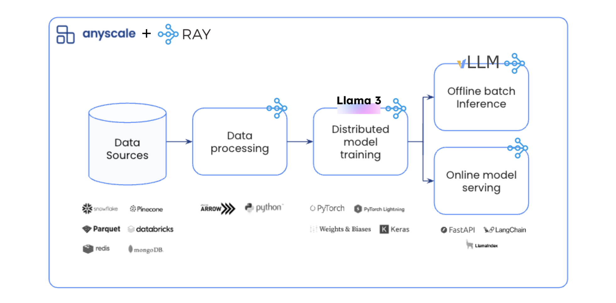
How are perplexities over multiple instance aggregated?
The perplexity of the $i^{th}$ token in the $k^{th}$ sequence is $$ P_{ki} = \frac{1}{p(t_{ki})} $$ The perplexity aggregated for the $k^{th}$ sequence is then $$ P_{k} = \left(\prod_{i=1}^N P_{ki}\right)^{1/N} \\ = \left(\prod_{i=1}^N \frac{1}{p(t_{ki})} \right)^{1/N} $$ which is the geometric mean of the perplexities of the tokens. This makes sense as we are essentially taking the multiplicative inverse of the probability that the model got the whole sequence correct. Now my question is how to aggregate the perplexities of several sequences. It seems from various places, including the Hugging Face Tutorial , I see that the prescription is to take the arithmetic mean of the perplexities of sequences $$ P = \frac{1}{m} \sum_{k=1}^m P_k $$ I am not quite understanding what it means to take the average of 1/probabilities. What is this actually capturing?
Experiments in Weak-to-Strong Generalization
Writing up results from a recent project
Moderator Analysis in Cox Regression
Imagine an RCT with two groups with a time-to-event endpoint. The (pre-specified) strategy for analysing this trial is a Cox Regression using common covariate adjustment to reduce outcome heterogeneity. So far, so good. Now I want to know whether my treatment effect is moderated by level of education (3 levels). If I used the pre-specified cox regression with covariate adjustment and integrated the treatment*education interaction, the SEs are getting very large. What may the reasons be? Is my sample size (120 per group) too little and should I reduce the covariates for which I adjust? Edit: I controlled for 4 covariates. There were 76 events in the IG and 91 events in the CG. More specifically: Education level1: IG: 13 CG: 18. Education level2: IG: 32 CG: 28. Education level3: IG: 31 CG: 45
Free Form Least-Squares Concept Erasure Without Oracle Concept Labels
Achieving even more surgical edits than LEACE without concept labels at inference time.
DDPG model outputting a fixed action at every timestep
I am trying to create a Car Following model, for which i am using DDPG. My action is acceleration bounded in a range of [-3,3] m/s2. While training the model, for every state it gives a single acceleration value i.e. 3 (or sometimes -3). It can be clearly seen that my actor is performing really bad. What can be done to resolve this issue?
Why work at the EU AI Office?
It's probably not for everyone, but there are a lot of great reasons to consider, including the potential to have an impact on AI governance worldwide, leveraging the first-mover advantage, and more.
Would the DDPG algorithm still function effectively if some transitions stored in its replay buffer are generated by a completely unrelated policy?
Let's hypothesize a scenario where some of the records ( s i , a i , r i , s i+1 ) in the replay buffer are generated by another completely unrelated random policy. If the DDPG algorithm still samples random minibatches from this buffer for learning as usual, would the learning process proceed successfully? Actually, there's a pre-processing stage before training DDPG in my online learning application, where another module learns the safe action range. I wonder if the transition records obtained during this stage can be used to pre-train the DDPG agent.
Q&A: Discover what’s new in the Mobile Payments SDK beta
Learn about how KIOS, a kiosk software, conducted early stage testing of the SDK and their integration experience.